Brownian Motion Part II

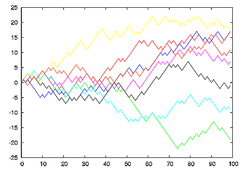
As I said in my last post regarding the section in which we were discussing Brownian motion, I was working on using mathematica to graph an illsutration of what Brownian motion looked like. As we discussed in class it looks very much like a Stock Market diagram (and in fact Brownian Motion is a large part of Economics and Finance). I was able to complete this task and constructed a graph of a random walk to illustrate Brownian motion in one dimension.

• One Dimensional "Drunkards Walk"

• In the example above the points are disconnected, but since they are so close together, you can still see the outline of the graph.
• In the example below I have connected the points and exectued the same piece of code. Each time it is executed, a new graph is formed due to the natural randomness of brownian motion.

• Code:
  RandomWalk[n_] := NestList[(# + (-1)^Random[Integer]) &, 0, n];
  ListPlot[RandomWalk[3000], PlotJoined -> True]

This is a cool website I came across with small applets showing both one and two dimensional brownian motion: Click Here

In class we did a sort of extended proof that Brownian motion exists (about 2.5 class sessions). This proof had, what seemed to be quite a bit of statistics involved in it and I will not attempt to rewrite the 5 pages of notes I have on it in this blog. I will however discuss what I got out of those classes:

1. Brownian motion exists.
   This was the conclusion we came to in our extended proof.
2. The paths of Brownian motion are continuous.
   This would be fairly easy to justify with the definition of continous.
3. The paths are non-differentiable anywhere.
   Holy cow! Continous, but not differentiable anwhere?
4. The paths to Brownian motion are fractals.
   Ah, yes. What I was waiting for all along, a tie in to fractals. This webpage made this part a little more clear in my eyes. It states that Brownian motion is self-similar in law, then has an applet which zooms in continuously on a random walk. You can see that the graph stretches a bit, but keeps it's generaly shape no matter how much you zoom in.
   

Correction to Bifurcation Diagram

In assignment #1 we were asked about the Iterated function system:

x(n+1) = f(x(n))
where f(x) = Cx(1-x), for some range of values for C

I had been coding this incorrectly in mathematica, I recently found out how to code it correctly, and thusly would like to make some corrections to my conclusions about this assignment.
Code:

g[x_] := a x (1 - x);
plist = {};
Do[x = 0.3; Do[x = g[x], {1000}];
Do[x = g[x]; plist = Append[plist, {a, x}], {1000}], {a, 2.8, 4, 10^-2}];
ListPlot[plist];


Approximately what range of C gives you chaos?

• Well as far as I can see the diagram looks more "chaotic" in the darker areas, and less chaotic in the white strips. Upon first look when C <~ 3.48 the graph just looks like a binary tree that keeps branching off two at a time, after that it becomes somewhat of a mess. The diagram does seem to have certain "jumps" though, where it clears up from time to time.

Approximately what range of C does not give you chaos?

• This diagram is definitely not chaotic before C = 3.48. After that it seems like it alternates between chaos and white space. If you zoom in on certain parts, you can see a simlilar pattern to the graph where C <>

Do you see any fractals?

• Yes. I see some self similarity anyway. This leads me to believe that there are fractals in this mapping.

Do you see a connection between chaos and fractals?

• There is obviously a connection between these two things, whenever there are fractals, chaos seems to be lurking around somewhere, be it in the form of randomness (i.e. Brownian motion) or the dark areas that seemingly come out of nowhere in this bifurcation mapping.

Brownian Motion

For the past couple weeks in class we have spent a lot of time discussing (and trying to prove) Brownian motion and it's characteristics. While very interesting, this topic came off to me as quite abstract and difficult to picture in my head. It inolves a lot of probability and took some statistical background knowledge to follow the lecture.

The first subtopic which we came across that I had some trouble understanding was "random walk". After I researched this a little bit I found that it is also called a "drunkards walk" and looks something like this:

1. Start at some given point
2. Move forward to another point in some direction (chosen at random) with each direction having the same probability.

Here is an example showing eight different "drunkards walks" with 100 timesteps (points) each:

Not as symmetric or pleasing to the eye as the other graphics we've looked at prior too this section, but important nonetheless.

I also took some time to try and learn to make a random walk using Mathematica, and will post my results (*here*) when I finish.

From what I can tell, Brownian motion is simply a specific type of random walk, which has to do with the diffusion process of certain particles. I found this graphic of Brownian motion:

Once again not the most pleasing to the eye, but I guess that's why its "random" motion. As I review I'll post the proof we composed of the existence of Brownian motion.

Assignmnent: Problem 1 from syllabus

Problem number 1) from the syllabus page of the website is stated as
1) Consider the iteration , x(n+1)=f(x(n)), where f(x) = Cx(1-x), for various different values of C. Approximately what range of C gives you chaos? Approximately what range of C does not give you chaos? Do you see any fractals? Do you see any evidence of a connection between chaos and fractals?

As far as I can see -2<4>

• C = -1:

• C=1:

• C=2:

• C=3:

I wasn't able to recognize any fractals when investigating this IFS. This may be because of the initial condition I used (x(0) = 0.3). I also can't put together the link between chaos and fractals as of this time.

Assignment: Feathered Fractal (Toy)

This fractal is similar to a Cantor set. It has no overlaps and comes from the map of the union of two transformations f and g.

This is the code I used in Mathematica:

This is the fractal, broken down between 10 iterations of the transformation:

This is the graph after 15 iterations:

Assignment (Binary String vs. IFS)

This assignment was stated as follows:

Consider the chaotic iteration x(n+1)=f(x(n)), where f(x) = 4x(1-x), and initial condition x(0)= 0.3. Is the sequence of numbers x(n) for n=0,1,2,3,4, . . . random or deterministic? Now consider the function h(x) defined by h(x)=0 for x<0.5>h(x)=1 for x>=0.5, and also consider the sequence of bits y(n)=h(x(n)), where x(n) comes from the chaotic iteration above. Is the sequence y(n) deterministic or random? Here are two sequences of bits, each 1000 steps long. One sequence comes from a chaotic iteration for a certain choice of intial condition, the other is random (or is it?). Can you tell the difference? Which is which?

As for the first part of the assignment, to find whether the sequence was random or deterministic I used Mathematica to make a plot of the system, this it what it looked like:
This leads me to believe that it was not deterministic. There doesn't exactly look as if there is much rhyme or reason to where the points are mapped to. Some spots on the graph look as if there is a pattern trying to emerge (i.e. the white spots along between .6 and .8 along the horizontal), but I'm not convinced that it shows the IFS to be deterministic.

As for the second part of this problem, we were to determine whether a mapping of this IFS onto a binary string would be deterministic or random and to find the difference between a random string and a string mapped from an IFS with a specific initial condition.

This was fairly difficult for me, but to do this I used Mathematica to help me determine which was which. First I copied our 2 given binary strings into separate lists in Mathematica.

• List a) had 510 zeros and 490 ones
  

• List b) had 495 zeros and 505 ones

This was not very helpful in finding which was the "random" string and which was produced through the IFS, since both are so close to 50% zeros and 50% ones, which would be what you might think the random string would have to be. I next created a function in Mathematica equal to the function given above and began guessing initial conditions to start with and iterating 1000 times, then mapping the list using the parameters given for h(x). Finally I subtracted this list from each of our given binary strings, and stopped once Mathematica gave a list of all zeros.

This is what the input and output looked like: {v4 being List b) from problem 2}

Thus, List a) is the coin flip, and List b) is x(n+1) = f(x(n)) with initial condition x(0) = 0.3
I can't say that I think this IFS mapped to a binary string using h(x) is deterministic. The outcome is very close to 50% of each number which is very close to the probability of a random number generator spitting out either 1 or 0.

Fractal dimension of a fractal determines its complexity. (What does this mean?)

This was a tough one. I feel like everything that has to do with fractals is very ambiguously defined. Even the definition of a fractal seems to be up in the air, defined with more, or less parameters depending on who or what your source is.

Upon first look at the statement,"the fractal dimension of an object determines its complexity" I would have to think that the fractal dimension has something to do with how intricate the rendering of the fractal is from a visual standpoint. When I think of the word complex it leads me to thinking that something looks confusing, or is dense with information. Thus, I believe the actual confusion lies on the word, complex. What does it mean?

The Oxford Dictionary defines something as "complex" if it "is made of closely connected parts". This could mean that something would be more complex if it had more closely connected parts. I believe this gives us a good realization of what the "complexity of a fractal" could mean.

Filling out the fractal

Yesterday, class was spent discussing how a fractal was filled. This was a very interesting lecture that helped me understand more how fractals will take shape and what they are composed of. Using an algorithm we were introduced to in the class prior, namely:

T' = T_1(A) U T_2(A) ; where A is a set such that
A = {x}

The iterations look something like this

{x} -> {T_1(x), T_2(x)} -> {(T_1)^2(x), T_1T_2(x), (T_2)^2(x)} ->...

and the transformations look like this

T_1(x,y) = |.5 .5, 0 .5| (x, y)


T_2(x, y) = |.5 .5, 0 .5| (x, y) + (0, .5)


At first we tried to perform these transformations on the unit square. This didn't work out because the first iteration of the transformation left no gap in between the subsequent skewed graphs , which as an effect caused the iterations to become static. We then decided to start with a square starting at the origin , going out 2 units in each direction. This caused the first transformation to have a small gap between the 2 parallelograms (the result of the first interation). This allows us to iterate infinitely.

At this point in the lecture we began discussing the idea of a point's address. That is, any point which is an element of the fractal can be assigned a distinct address. An address is a binary string of numbers that you can disect to find out exactly where this point is inside our fractal. For the specific fractal we were looking at, the first index of the address is assigned a 0 if it is on the bottom half of the original square or a one if it is on the top half. The second index of the address is assigned a 0 if it is on the bottom half of the parallelogram created for the first iteration of the transformation, and a 1 if it is on the top half. This is repeated a finite amount of times until you get the address of the exact point you are looking at.

The concept of address will be a little easier to understand if I can post the graph of the fractal we were examaning. As soon as I figure out how to graph it in mathematica, I 'll post the image.

Contracting Mapping

The better part of today's class was spent proving a theorem, which after a little bit of search I found is called the "Banach Fixed Point Theorem".

Banach Fixed Point Theorem:

Let (Y,m) me a complete metric space. Let T: Y -> Y be a continuous map such that for all x,y that are elements of Y, m(Tx,Ty) <= km(x,y) for some |k|<1.> x'.

From Mathworld:

Let be a contraction mapping from a closed subset of a Banach space into . Then there exists a unique such that .

My take on this:

It is easier for me to understand the theorem given to us in class rather than the theorem I found on Mathworld. (Maybe because I have no idea what "Banach space" is.) The way I see this is thatt T is a contracting transformation (which is the reason 0<1) style="font-weight: bold;">Summation of the Proof:

We proved this in 2 parts:

1. There is only 1 fixed point. This was proved by assuming there are 2 and showing they are equal. To do this we had to assume the sequence {(T^n)(y)} is cauchy.
   
2. Prove that the previous sequence is cauchy.

Convergent Series

Back on the 10th, we were given the assignment to find the value of 3 different sums (series).

The first of which was the sum of (1/(2^i)) as i goes from zero to infinity. The number that this series will eventually converge to is 2.

Next we had to find the sum of (1/(2^i)) as i goes from 1 to infinity. This converges to 1.

The last series we were assigned to evalute was the sum of (1/(2^i)) as i goes from 2 to infinity. As far as I can see this should converge to 1/2.

Proof:

1)

The n-th partial sum for this series is defined as
S _n = 1/2 + 1/2 ² + 1/2 ³ + ... + 1/2 n

If we divide the above expression by 2 and then subtract it from the original one we get:

S _n - 1/2 S _n = 1/2 - 1/2 ⁿ⁺¹

Hence, solving this for S _n we obtain

S _n = 2 (1/2 - 1/2 ⁿ⁺¹)

This is now a sequence, and we can take the limit as n goes to infinity. By our result on the power sequence, the term 1/2 ⁿ⁺¹ goes to zero,
so that lim S _n = 1

Taken From:
Interactive Real Analysis, ver. 1.9.4
(c) 1994-2005, Bert G. Wachsmuth

2) For the same series but with n starting at 0 or 2 we can just add or subtract the singleton element from our series limit. i.e. if we start with n=0, then one more element will be added to the series. The element 1/(2^0) = 1, so the limit as n goes to infinity is 1+1=2. On the other hand if we start with one less element such that n=2, then we can subtract the element 1/(2^1)=1/2, thus our limit would be 1-1/2=1/2.